Here is updated spreadsheet to help working out who to trade in or out of your team to get the best money changes after the end of round 3 and 4.
Brief instructions:
- You only have to enter information into the green cells, the other cells are protected to prevent any errors.
- Confirm or change Magic Number estimate for the end of round 3 – cell U2. I’ve put it at 5,050 – if you think you know enough about MN to put another number you can change it. Similar for MN at end of round 4 – I have it at 4,950.
- Enter your players using the drop down menu. In the menu only the players who fit that position are named in full, other players are reduced to 3 letters. If you used the spreadsheet from Round 1 you should be able to select and copy groups of players from there into this spreadsheet.
- For each player in your team data is pulled up automatically –
- Team and position for 2013. If this is different to 2012, their previous team and position is also shown, or if this is their 1st year playing.
- 2013 starting price.
- Points expected based on that price (using initial magic number 5,150).
- The difference in points between their 2013 base and their points average for all of 2012. For most players who played last year this difference will be zero.
- 2012 Performance in 3 columns – average points, games played, standard deviation.
- Scores from the first 2 rounds – “n” indicates they did not play.
- There are 2 green cells to enter the actual scores (or your estimates) for your players for the Round 3 and Round 4. Based on these scores the last other columns calculate the averages, BEs, price change and new prices after the rounds.
- If you leave any cell blank the calculation assumes the player gets their 2013 base score for that round – i.e. the score in column G is used as default in the calculations. The default is not the player’s current average score.
- The player has to play 3 games for their price to change, so if the players miss games their price change won’t happen until after they play 3 games.
- The captain’s score isn’t doubled so the total score won’t match your real DT score for the rounds.
At the bottom of the spreadsheet there are 2 more tables. One table looks at the structure of your team, the other looks at distribution of byes.
Here is link to download spreadsheet (excel2007) – DT2013 R3pub
If you have any questions, post comments below or tweet to @NixTrader
FAQ:
- Why are these calculations different to other published BEs and valuations?
- Everyone’s calculations depend on their assumptions about Magic Number, projections of future scores and how they round averages and values. This spreadsheet should replicate any other published calculations if you make the same projections, including changing the magic number. However, this spreadsheet is unique in that it allows you to change the estimates to do your own analysis.
- Tech talk: You need a device that supports microsoft excel 2007 spreadsheets to be able to open and use the spreadsheet. It won’t open on mobiles or tablets unless you have software or apps that support excel files.
EDIT:
- If one of your players misses round 3, put an “n” in the green cell for that round. The calculations for round 4 will then update to take account of this. If you leave R3 blank the default assumption is that the player does play in R3 and scores the amount in column G.


Recent Comments